Pandas
Questions
How do I learn a new Python package?
How can I use pandas dataframes in my research?
Objectives
Learn simple and some more advanced usage of pandas dataframes
Get a feeling for when pandas is useful and know where to find more information
Understand enough of pandas to be able to read its documentation.
Pandas is a Python package that provides high-performance and easy to use data structures and data analysis tools. This page provides a brief overview of pandas, but the open source community developing the pandas package has also created excellent documentation and training material, including:
A Getting started guide (including tutorials and a 10 minute flash intro)
A “10 minutes to Pandas” tutorial
Thorough Documentation containing a user guide, API reference and contribution guide
A cookbook
A quick Pandas preview
Let’s get a flavor of what we can do with pandas (you won’t be able to follow everything yet). We will be working with an example dataset containing the passenger list from the Titanic, which is often used in Kaggle competitions and data science tutorials. First step is to load pandas:
import pandas as pd
We can download the data from this GitHub repository
by visiting the page and saving it to disk, or by directly reading into
a DataFrame:
url = "https://raw.githubusercontent.com/pandas-dev/pandas/master/doc/data/titanic.csv"
titanic = pd.read_csv(url, index_col='Name')
We can now view the dataframe to get an idea of what it contains and print some summary statistics of its numerical data:
# print the first 5 lines of the dataframe
titanic.head()
# print summary statistics for each column
titanic.describe()
Ok, so we have information on passenger names, survival (0 or 1), age, ticket fare, number of siblings/spouses, etc. With the summary statistics we see that the average age is 29.7 years, maximum ticket price is 512 USD, 38% of passengers survived, etc.
Let’s say we’re interested in the survival probability of different
age groups. With two one-liners, we can find the average age of those
who survived or didn’t survive, and plot corresponding histograms of
the age distribution (pandas.DataFrame.groupby(), pandas.DataFrame.hist()):
print(titanic.groupby("Survived")["Age"].mean())
titanic.hist(column='Age', by='Survived', bins=25, figsize=(8,10),
             layout=(2,1), zorder=2, sharex=True, rwidth=0.9);
Clearly, pandas dataframes allows us to do advanced analysis with very few commands, but it takes a while to get used to how dataframes work so let’s get back to basics.
Getting help
Series and DataFrames have a lot functionality, but
how can we find out what methods are available and how they work? One way is to visit
the API reference
and reading through the list.
Another way is to use the autocompletion feature in Jupyter and type e.g.
titanic["Age"]. in a notebook and then hit TAB twice - this should open
up a list menu of available methods and attributes.
Jupyter also offers quick access to help pages (docstrings) which can be more efficient than searching the internet. Two ways exist:
Write a function name followed by question mark and execute the cell, e.g. write
titanic.hist?and hitSHIFT + ENTER.Write the function name and hit
SHIFT + TAB.Right click and select “Show contextual help”. This tab will update with help for anything you click.
What’s in a dataframe?
As we saw above, pandas dataframes are a powerful tool for working with tabular data.
A pandas
pandas.DataFrame
is composed of rows and columns:

Each column of a dataframe is a pandas.Series object
- a dataframe is thus a collection of series:
# print some information about the columns
titanic.info()
Unlike a NumPy array, a dataframe can combine multiple data types, such as
numbers and text, but the data in each column is of the same type. So we say a
column is of type int64 or of type object.
Let’s inspect one column of the Titanic passenger list data (first downloading and reading the titanic.csv datafile into a dataframe if needed, see above):
titanic["Age"]
titanic.Age          # same as above
type(titanic["Age"]) # a pandas Series object
The columns have names. Here’s how to get them (columns):
titanic.columns
However, the rows also have names! This is what Pandas calls the index:
titanic.index
We saw above how to select a single column, but there are many ways of
selecting (and setting) single or multiple rows, columns and
values. We can refer to columns and rows either by their name
(loc, at) or by
their index (iloc,
iat):
titanic.loc['Lam, Mr. Ali',"Age"]          # select single value by row and column
titanic.loc[:'Lam, Mr. Ali',"Survived":"Age"]  # slice the dataframe by row and column *names*
titanic.iloc[0:2,3:6]                      # same slice as above by row and column *numbers*

titanic.at['Lam, Mr. Ali',"Age"] = 42      # set single value by row and column *name* (fast)
titanic.at['Lam, Mr. Ali',"Age"]           # select single value by row and column *name* (fast)
titanic.iat[0,5]                           # select same value by row and column *number* (fast)

titanic["is_passenger"] = True             # set a whole column
Dataframes also support boolean indexing, just like we saw for numpy
arrays:
titanic[titanic["Age"] > 70]
# ".str" creates a string object from a column
titanic[titanic.index.str.contains("Margaret")]
What if your dataset has missing data? Pandas uses the value numpy.nan
to represent missing data, and by default does not include it in any computations.
We can find missing values, drop them from our dataframe, replace them
with any value we like or do forward or backward filling:
titanic.isna()                    # returns boolean mask of NaN values
titanic.dropna()                  # drop missing values
titanic.dropna(how="any")         # or how="all"
titanic.dropna(subset=["Cabin"])  # only drop NaNs from one column
titanic.fillna(0)                 # replace NaNs with zero
titanic.fillna(method='ffill')    # forward-fill NaNs
Exercises 1
Exploring dataframes
Have a look at the available methods and attributes using the API reference or the autocomplete feature in Jupyter.
Try out a few methods using the Titanic dataset and have a look at the docstrings (help pages) of methods that pique your interest
Compute the mean age of the first 10 passengers by slicing and the
pandas.DataFrame.mean()method(Advanced) Using boolean indexing, compute the survival rate (mean of “Survived” values) among passengers over and under the average age.
Solution
Mean age of the first 10 passengers:
titanic.iloc[:10,:]["Age"].mean()
or:
titanic.loc[:"Nasser, Mrs. Nicholas (Adele Achem)","Age"].mean()
or:
titanic.iloc[:10,4].mean()
Survival rate among passengers over and under average age:
titanic[titanic["Age"] > titanic["Age"].mean()]["Survived"].mean()
and:
titanic[titanic["Age"] < titanic["Age"].mean()]["Survived"].mean()
Tidy data
The above analysis was rather straightforward thanks to the fact that the dataset is tidy.
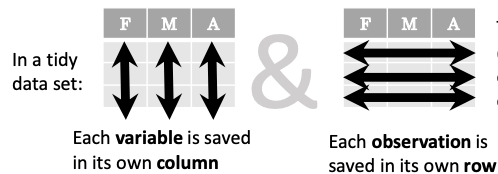
In short, columns should be variables and rows should be measurements, and adding measurements (rows) should then not require any changes to code that reads the data.
What would untidy data look like? Here’s an example from some run time statistics from a 1500 m running event:
runners = pd.DataFrame([
              {'Runner': 'Runner 1', 400: 64, 800: 128, 1200: 192, 1500: 240},
              {'Runner': 'Runner 2', 400: 80, 800: 160, 1200: 240, 1500: 300},
              {'Runner': 'Runner 3', 400: 96, 800: 192, 1200: 288, 1500: 360},
          ])
What makes this data untidy is that the column names 400, 800, 1200, 1500 indicate the distance ran. In a tidy dataset, this distance would be a variable on its own, making each runner-distance pair a separate observation and hence a separate row.
To make untidy data tidy, a common operation is to “melt” it, which is to convert it from wide form to a long form:
runners = pd.melt(runners, id_vars="Runner",
              value_vars=[400, 800, 1200, 1500],
              var_name="distance",
              value_name="time"
          )
In this form it’s easier to filter, group, join and aggregate the data, and it’s also easier to model relationships between variables.
The opposite of melting is to pivot data, which can be useful to view data in different ways as we’ll see below.
For a detailed exposition of data tidying, have a look at this article.
Working with dataframes
We saw above how we can read in data into a dataframe using the read_csv() function.
Pandas also understands multiple other formats, for example using read_excel,
read_hdf, read_json, etc. (and corresponding methods to write to file:
to_csv, to_excel, to_hdf, to_json, etc.)
But sometimes you would want to create a dataframe from scratch. Also this can be done
in multiple ways, for example starting with a numpy array (see
DataFrame docs):
import numpy as np
dates = pd.date_range('20130101', periods=6)
df = pd.DataFrame(np.random.randn(6, 4), index=dates, columns=list('ABCD'))
df
or a dictionary (see same docs):
df = pd.DataFrame({'A': ['dog', 'cat', 'dog', 'cat', 'dog', 'cat', 'dog', 'dog'],
                   'B': ['one', 'one', 'two', 'three', 'two', 'two', 'one', 'three'],
                   'C': np.array([3] * 8, dtype='int32'),
                   'D': np.random.randn(8),
                   'E': np.random.randn(8)})
df
There are many ways to operate on dataframes. Let’s look at a few examples in order to get a feeling of what’s possible and what the use cases can be.
We can easily split and concatenate dataframes:
sub1, sub2, sub3 = df[:2], df[2:4], df[4:]
pd.concat([sub1, sub2, sub3])
When pulling data from multiple dataframes, a powerful pandas.DataFrame.merge method is
available that acts similarly to merging in SQL. Say we have a dataframe containing the age of some athletes:
age = pd.DataFrame([
    {"Runner": "Runner 4", "Age": 18},
    {"Runner": "Runner 2", "Age": 21},
    {"Runner": "Runner 1", "Age": 23},
    {"Runner": "Runner 3", "Age": 19},
])
We now want to use this table to annotate the original runners table from
before with their age. Note that the runners and age dataframes have a
different ordering to it, and age has an entry for Dave which is not
present in the runners table. We can let Pandas deal with all of it using
the merge method:
# Add the age for each runner
runners.merge(age, on="Runner")
In fact, much of what can be done in SQL is also possible with pandas.
groupby is a powerful method which splits a dataframe and aggregates data
in groups. To see what’s possible, let’s return to the Titanic dataset. Let’s
test the old saying “Women and children first”. We start by creating a new
column Child to indicate whether a passenger was a child or not, based on
the existing Age column. For this example, let’s assume that you are a
child when you are younger than 12 years:
titanic["Child"] = titanic["Age"] < 12
Now we can test the saying by grouping the data on Sex and then creating further sub-groups based on Child:
titanic.groupby(["Sex", "Child"])["Survived"].mean()
Here we chose to summarize the data by its mean, but many other common
statistical functions are available as dataframe methods, like
std, min,
max, cumsum,
median, skew,
var etc.
Exercises 2
Analyze the Titanic passenger list dataset
In the Titanic passenger list dataset, investigate the family size of the passengers (i.e. the “SibSp” column).
What different family sizes exist in the passenger list? Hint: try the
unique()methodWhat are the names of the people in the largest family group?
(Advanced) Create histograms showing the distribution of family sizes for passengers split by the fare, i.e. one group of high-fare passengers (where the fare is above average) and one for low-fare passengers (Hint: instead of an existing column name, you can give a lambda function as a parameter to
hist()to compute a value on the fly. For examplelambda x: "Poor" if df["Fare"].loc[x] < df["Fare"].mean() else "Rich").
Solution
Existing family sizes:
titanic["SibSp"].unique()
We get 8 from above. There is no
Namecolumn, since we madeNamethe index when we loaded the dataframe withread_csv, so we usepandas.DataFrame.indexto get the names. So, names of members of largest family(ies):titanic[titanic["SibSp"] == 8].index
Histogram of family size based on fare class:
titanic.hist("SibSp",
             lambda x: "Poor" if titanic["Fare"].loc[x] < titanic["Fare"].mean() else "Rich",
             rwidth=0.9)
Time series superpowers
An introduction of pandas wouldn’t be complete without mention of its special abilities to handle time series. To show just a few examples, we will use a new dataset of Nobel prize laureates available through an API of the Nobel prize organisation at https://api.nobelprize.org/v1/laureate.csv .
Unfortunately this API does not allow “non-browser requests”, so
pandas.read_csv will not work directly on it. Instead, we put a
local copy on Github which we can access (the original data is CC-0,
so we are allowed to do this). (Aside: if you do JupyterLab →
File → Open from URL → paste the URL above, it will open it in
JupyterLab and download a copy for your use.)
We can then load and explore the data:
nobel = pd.read_csv("https://github.com/AaltoSciComp/python-for-scicomp/raw/master/resources/data/laureate.csv")
nobel.head()
This dataset has three columns for time, “born”/”died” and “year”.
These are represented as strings and integers, respectively, and
need to be converted to datetime format. pandas.to_datetime()
makes this easy:
# the errors='coerce' argument is needed because the dataset is a bit messy
nobel["born"] = pd.to_datetime(nobel["born"], errors ='coerce')
nobel["died"] = pd.to_datetime(nobel["died"], errors ='coerce')
nobel["year"] = pd.to_datetime(nobel["year"], format="%Y")
Pandas knows a lot about dates (using .dt accessor):
print(nobel["born"].dt.day)
print(nobel["born"].dt.year)
print(nobel["born"].dt.weekday)
We can add a column containing the (approximate) lifespan in years rounded to one decimal:
nobel["lifespan"] = round((nobel["died"] - nobel["born"]).dt.days / 365, 1)
and then plot a histogram of lifespans:
nobel.hist(column='lifespan', bins=25, figsize=(8,10), rwidth=0.9)
Finally, let’s see one more example of an informative plot (boxplot())
produced by a single line of code:
nobel.boxplot(column="lifespan", by="category")
Exercises 3
Analyze the Nobel prize dataset
What country has received the largest number of Nobel prizes, and how many? How many countries are represented in the dataset? Hint: use the
describemethod on thebornCountryCodecolumn.Create a histogram of the age when the laureates received their Nobel prizes. Hint: follow the above steps we performed for the lifespan.
List all the Nobel laureates from your country.
Now more advanced steps:
Now define an array of 4 countries of your choice and extract only laureates from these countries (you need to look at the data and find how countries are written, and replace
COUNTRYwith those strings):countries = np.array([COUNTRY1, COUNTRY2, COUNTRY3, COUNTRY4]) subset = nobel.loc[nobel['bornCountry'].isin(countries)]Use
groupby()to compute how many nobel prizes each country received in each category. Thesize()method tells us how many rows, hence nobel prizes, are in each group:nobel.groupby(['bornCountry', 'category']).size()(Optional) Create a pivot table to view a spreadsheet like structure, and view it
First add a column “number” to the nobel dataframe containing 1’s (to enable the counting below). We need to make a copy of
subset, because right now it is only a view:subset = subset.copy() subset.loc[:, 'number'] = 1Then create the
pivot_table():table = subset.pivot_table( values="number", index="bornCountry", columns="category", aggfunc="sum" )(Optional) Install the
seabornvisualization library if you don’t already have it, and create a heatmap of your table:import seaborn as sns sns.heatmap(table,linewidths=.5);(Optional) Play around with other nice looking plots:
sns.violinplot(y=subset["year"].dt.year, x="bornCountry", inner="stick", data=subset);sns.swarmplot(y="year", x="bornCountry", data=subset, alpha=.5);subset_physchem = nobel.loc[ nobel['bornCountry'].isin(countries) & ( nobel['category'].isin(['physics']) | nobel['category'].isin(['chemistry']) ) ] sns.catplot( x="bornCountry", y="year", col="category", data=subset_physchem, kind="swarm" );sns.catplot(x="bornCountry", col="category", data=subset_physchem, kind="count");
Solution
Below is solutions for the basic steps, advanced steps are inline above.
We use the describe() method:
nobel.bornCountryCode.describe()
# count     969
# unique     82
# top        US
# freq      292
We see that the US has received the largest number of Nobel prizes, and 82 countries are represented.
To calculate the age at which laureates receive their prize, we need to ensure that the “year” and “born” columns are in datetime format:
nobel["born"] = pd.to_datetime(nobel["born"], errors ='coerce')
nobel["year"] = pd.to_datetime(nobel["year"], format="%Y")
Then we add a column with the age at which Nobel prize was received and plot a histogram:
nobel["age_nobel"] = round((nobel["year"] - nobel["born"]).dt.days / 365, 1)
nobel.hist(column="age_nobel", bins=25, figsize=(8,10), rwidth=0.9)
We can print names of all laureates from a given country, e.g.:
nobel[nobel["country"] == "Sweden"].loc[:, "firstname":"surname"]
Beyond the basics
Faster expression evaluation with eval()
Larger DataFrame operations might be faster using eval() with string expressions (see
here).
To do so, we start by installing numexpr a Python library which optimizes such expressions:
%conda install numexpr
You may need to restart the kernel in Jupyter for this to be. Then:
import pandas as pd
import numpy as np

# Make some really big dataframes
nrows, ncols = 100000, 100
rng = np.random.RandomState(42)
df1, df2, df3, df4 = (pd.DataFrame(rng.rand(nrows, ncols))
                      for i in range(4))
Adding dataframes the pythonic way yields:
%timeit df1 + df2 + df3 + df4
# 80ms
And by using eval():
%timeit pd.eval('df1 + df2 + df3 + df4', engine='numexpr')
# 40ms
Assigning columns with apply()
We can assign function return lists as dataframe columns:
def fibo(n):
    """Compute Fibonacci numbers. Here we skip the overhead from the
    recursive function calls by using a list. """
    if n < 0:
        raise NotImplementedError('Not defined for negative values')
    elif n < 2:
        return n
    memo = [0]*(n+1)
    memo[0] = 0
    memo[1] = 1
    for i in range(2, n+1):
        memo[i] = memo[i-1] + memo[i-2]
    return memo

df = pd.DataFrame({'Generation': np.arange(100)})
df['Number of Rabbits'] = fibo(99)  # Assigns list to column
There is much more to Pandas than what we covered in this lesson. Whatever your
needs are, chances are good there is a function somewhere in its API. You should try to get good at
searching the web for an example showing what you can do. And when
there is not, you can always
apply your own functions to the data using apply:
from functools import lru_cache

@lru_cache
def fib(x):
    """Compute Fibonacci numbers. The @lru_cache remembers values we
    computed before, which speeds up this function a lot."""
    if x < 0:
        raise NotImplementedError('Not defined for negative values')
    elif x < 2:
        return x
    else:
        return fib(x - 2) + fib(x - 1)

df = pd.DataFrame({'Generation': np.arange(100)})
df['Number of Rabbits'] = df['Generation'].apply(fib)
Note that the numpy precision for integers caps at int64 while python ints are unbounded –
limited by memory size. Thus, the result from fibonacci(99) would be erroneous when
using numpy ints. The type of df['Number of Rabbits'][99] given by both functions above
is in fact <class 'int'>.
See also
Modern Pandas (2020) – a blog series on writing modern idiomatic pandas.
Python Data Science Handbook (2016) – which contains a chapter on Data Manipulation with Pandas.
Alternatives to Pandas
Polars
Polars is a DataFrame library designed to processing data with a fast lighting time. Polars is implemented in Rust Programming language and uses Apache Arrow as its memory format.
Dask
Dask is a Python package for parallel computing in Python and uses parallel data-frames for dealing with very large arrays.
Vaex
Vaex is a high performance Python library for lazy Out-of-Core DataFrames, to visualize and explore big tabular datasets.
Keypoints
pandas dataframes are a good data structure for tabular data
Dataframes allow both simple and advanced analysis in very compact form