Profiling

Objectives

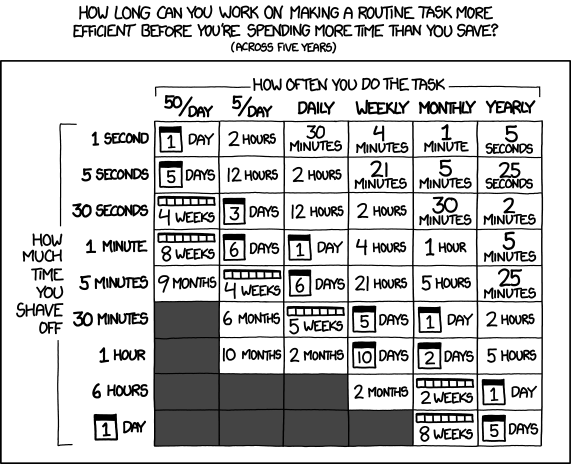
Understand when improving code performance is worth the time and effort.
Knowing how to find performance bottlenecks in Python code.
Try scalene as one of many tools to profile Python code.

Instructor note

Discussion: 20 min
Exercise: 20 min

Should we even optimize the code?

Classic quote to keep in mind: “Premature optimization is the root of all evil.” [Donald Knuth]

Humorous comic from xkcd that shows how long you can work on making a routine task more efficient before you're spending more time than you save? — Figure 1: Is it worth the time? (xkcd#1205)

Discussion

It is important to ask ourselves whether it is worth it.

Is it worth spending e.g. 2 days to make a program run 20% faster?
Is it worth optimizing the code so that it spends 90% less memory?

Depends. What does it depend on?

Key steps of optimization

When you encounter a situation that you think would benefit from optimization, follow these three steps:

Measure: Before doing blind modifications you should figure out which part of the code is actually the problem.

This is analogous to medical doctors doing lab tests and taking X-rays to determine the disease. They won’t start treatment without figuring out what is wrong with the patient.
Diagnose: When you have found out the part of the code that is slow, you should determine why it is slow. Doing changes without knowing why the code is slow can be counter-productive. Remember that not all slow parts can be endlessly optimized: some parts of the code might take time because they do a lot of work.

This step is analogous to doctor creating a specialized treatment program for a disease.
Treat: When you have found out the slow part and figured what causes it to be slow, you can then try to fix it.

This is analogous to doctor treating the disease with surgery or a prescription.

Using profiling to measure your program

While diagnosing and treating depends heavily on the case at hand, the measurement part can be done with tools and tactics that show where the bottlenecks are. This is called profiling.

Doing profiling is recommended for everyone. Even experienced programmers can be surprised by the results of profiling.

Scale matters for profiling

Sometimes we can configure the system size (for instance the time step in a simulation or the number of time steps or the matrix dimensions) to make the program finish sooner.

For profiling, we should choose a system size that is representative of the real-world use case. If we profile a program with a small input size, we might not see the same bottlenecks as when running the program with a larger input size.

Often, when we scale up the system size, or scale the number of processors, new bottlenecks might appear which we didn’t see before. This brings us back to: “measure instead of guessing”.

At the same time adding more time steps or more iterations can mean that the program does the same things over and over again. Thus sometimes you can try to profile a program for a shorter time and then extrapolate the results for the case where you’re running for a longer time. When doing this be mindful to profile enough so that you can make proper extrapolations.

Simplest profiling: timers

Simplest way of determining where the time-consuming parts are is to insert timers into your code:

import time

# ...
# code before the function

start = time.time()
result = some_function()
print(f"some_function took {time.time() - start} seconds")

# code after the function
# ...

An alternative solution that also improves your code’s output is to use Python’s logging module to log important breakpoints in your code. You can then check the timestamps of different log entries to see how long it took to execute a section of your code.

Better profiling: Dedicated profiling tools

There are plenty of dedicated profile tools that can be used to profile your code. These can measure the CPU time and memory utilization often on a line-by-line level.

The list below here is probably not complete, but it gives an overview of the different tools available for profiling Python code.

CPU profilers:

Memory profilers:

memory_profiler (not actively maintained)
Pympler
tracemalloc
guppy/heapy

CPU, memory and GPU:

Scalene

Tracing profilers vs. sampling profilers

Tracing profilers record every function call and event in the program, logging the exact sequence and duration of events.

Pros:
- Provides detailed information on the program’s execution.
- Deterministic: Captures exact call sequences and timings.
Cons:
- Higher overhead, slowing down the program.
- Can generate larger amount of data.

Sampling profilers periodically samples the program’s state (where it is and how much memory is used), providing a statistical view of where time is spent.

Pros:
- Lower overhead, as it doesn’t track every event.
- Scales better with larger programs.
Cons:
- Less precise, potentially missing infrequent or short calls.
- Provides an approximation rather than exact timing.

Analogy: Imagine we want to optimize the London Underground (subway) system

We wish to detect bottlenecks in the system to improve the service and for this we have asked few passengers to help us by tracking their journey.

Tracing: We follow every train and passenger, recording every stop and delay. When passengers enter and exit the train, we record the exact time and location.
Sampling: Every 5 minutes the phone notifies the passenger to note down their current location. We then use this information to estimate the most crowded stations and trains.

Example profiling case: throwing darts to calculate pi

Problem description

In this example we’ll profile the following Python code:

import random
import math

def calculate_pi(n_darts):
    hits = 0
    for n in range(n_darts):
        i = random.random()
        j = random.random()
        r = math.sqrt(i*i + j*j)
        if (r<1):
            hits += 1
    pi = 4 * hits / n_darts
    return pi

This code implements a well known example of the Monte Carlo method, where by throwing darts at a dartboard we can calculate an approximation for pi.

Diagram that shows a unit circle inside a square with side length 1 — Figure 2: The algorithm throws darts at a dartboard and estimates pi by calculating the ratio of hits to throws

Profiling the example

Let’s run this with %%time-magic and ten million throws:

%%timeit
calculate_pi(10_000_000)

1.07 s ± 30.3 ms per loop (mean ± std. dev. of 7 runs, 1 loop each)

We can then profile the code with either cProfile by using the %%prun magic. Here we tell the magic to sort the results by the total time used and to give us top 5 time users:

%%prun -s tottime -l 5

def calculate_pi(n_darts):
    hits = 0
    for n in range(n_darts):
        i = random.random()
        j = random.random()
        r = math.sqrt(i*i + j*j)
        if (r<1):
            hits += 1
    pi = 4 * hits / n_darts
    return pi 

calculate_pi(10_000_000)

         30000742 function calls (30000736 primitive calls) in 4.608 seconds

   Ordered by: internal time
   List reduced from 150 to 5 due to restriction <5>

   ncalls  tottime  percall  cumtime  percall filename:lineno(function)
        4    2.545    0.636    4.005    1.001 {built-in method time.sleep}
 20000000    1.091    0.000    1.091    0.000 {method 'random' of '_random.Random' objects}
 10000000    0.571    0.000    0.571    0.000 {built-in method math.sqrt}
        3    0.172    0.057    0.270    0.090 {method 'poll' of 'select.epoll' objects}
        1    0.148    0.148    0.233    0.233 <string>:1(calculate_pi)

The output shows that most of the time is used by the random.random and math.sqrt function calls. Those functions are called in every iteration of the loop, so the profile makes sense.

Naive optimization: switching to NumPy functions

A naive approach to optimization might be to simply switch to using NumPy functions instead of basic Python functions. The code would then look like this:

import numpy

def calculate_pi_numpy(n_darts):
    hits = 0
    for n in range(n_darts):
        i = numpy.random.random()
        j = numpy.random.random()
        r = numpy.sqrt(i*i + j*j)
        if (r<1):
            hits += 1
    pi = 4 * hits / n_darts
    return pi

However, if we do the same profiling, we’ll find out that the program is ten times slower. Something must have gone wrong.

Actual optimization: using vectorization

The reason for the bad performance is simple: we didn’t actually reduce the number of function calls, we just switched them to ones from NumPy. These function call have extra overhead because they have more complex logic compared to the standard library ones.

The actual speedup is right around the corner: switch from the costly for-loop to vectorized calls. NumPy’s functions can calculate all of the operations for all of our numbers in a single function call without the for-loop:

def calculate_numpy_fast(n_darts):
    i = numpy.random.random(n_darts)
    j = numpy.random.random(n_darts)
    r = numpy.sqrt(i*i + j*j)
    hits = (r < 1).sum() 
    pi = 4 * hits / n_darts
    return pi

%%prun -s tottime -l 5

def calculate_numpy_fast(n_darts):
    i = numpy.random.random(n_darts)
    j = numpy.random.random(n_darts)
    r = numpy.sqrt(i*i + j*j)
    hits = (r < 1).sum() 
    pi = 4 * hits / n_darts
    return pi

calculate_numpy_fast(10_000_000)

         664 function calls (658 primitive calls) in 0.225 seconds

   Ordered by: internal time
   List reduced from 129 to 5 due to restriction <5>

   ncalls  tottime  percall  cumtime  percall filename:lineno(function)
        1    0.202    0.202    0.205    0.205 <string>:1(calculate_numpy_fast)
        2    0.010    0.005    0.010    0.005 {method '__exit__' of 'sqlite3.Connection' objects}
      2/1    0.009    0.005    0.214    0.214 <string>:1(<module>)
        1    0.002    0.002    0.002    0.002 {method 'reduce' of 'numpy.ufunc' objects}
        1    0.001    0.001    0.010    0.010 history.py:92(only_when_enabled)

So vectorizing the code achieved around five times speedup.

Profiling with scalene

The previous example can also be profiled with scalene. Scalene is a sampling profiler and it can be run in Jupyter as well with %scrun (line-mode) and %%scalene (cell-mode).

Scalene will produce a nice looking output containing line-by-line profiling information.

Exercises

Exercise: Practicing profiling

In this exercise we will use the Scalene profiler to find out where most of the time is spent and most of the memory is used in a given code example.

Please try to go through the exercise in the following steps:

Make sure scalene is installed in your environment (if you have followed this course from the start and installed the recommended software environment, then it is).
Download Leo Tolstoy’s “War and Peace” from the following link (the text is provided by Project Gutenberg): https://www.gutenberg.org/cache/epub/2600/pg2600.txt (right-click and “save as” to download the file and save it as “book.txt”).
Before you run the profiler, try to predict in which function the code (the example code is below) will spend most of the time and in which function it will use most of the memory.
Save the example code as example.py and run the scalene profiler on the following code example and browse the generated HTML report to find out where most of the time is spent and where most of the memory is used:
```
$ scalene example.py
```
Alternatively you can do this (and then open the generated file in a browser):
```
$ scalene example.py --html > profile.html
```
You can find an example of the generated HTML report in the solution below.
Does the result match your prediction? Can you explain the results?

Example code (example.py):

"""
The code below reads a text file and counts the number of unique words in it
(case-insensitive).
"""
import re


def count_unique_words1(file_path: str) -> int:
    with open(file_path, "r", encoding="utf-8") as file:
        text = file.read()
    words = re.findall(r"\b\w+\b", text.lower())
    return len(set(words))


def count_unique_words2(file_path: str) -> int:
    unique_words = []
    with open(file_path, "r", encoding="utf-8") as file:
        for line in file:
            words = re.findall(r"\b\w+\b", line.lower())
            for word in words:
                if word not in unique_words:
                    unique_words.append(word)
    return len(unique_words)


def count_unique_words3(file_path: str) -> int:
    unique_words = set()
    with open(file_path, "r", encoding="utf-8") as file:
        for line in file:
            words = re.findall(r"\b\w+\b", line.lower())
            for word in words:
                unique_words.add(word)
    return len(unique_words)


def main():
    # book.txt is downloaded from https://www.gutenberg.org/cache/epub/2600/pg2600.txt
    _result = count_unique_words1("book.txt")
    _result = count_unique_words2("book.txt")
    _result = count_unique_words3("book.txt")


if __name__ == "__main__":
    main()

Solution

Result of the profiling run for the above code example. You can click on the image to make it larger.

Results:

Most time is spent in the count_unique_words2 function.
Most memory is used in the count_unique_words1 function.

Explanation:

The count_unique_words2 function is the slowest because it uses a list to store unique words and checks if a word is already in the list before adding it. Checking whether a list contains an element might require traversing the whole list, which is an O(n) operation. As the list grows in size, the lookup time increases with the size of the list.
The count_unique_words1 and count_unique_words3 functions are faster because they use a set to store unique words. Checking whether a set contains an element is an O(1) operation.
The count_unique_words1 function uses the most memory because it creates a list of all words in the text file and then creates a set from that list.
The count_unique_words3 function uses less memory because it traverses the text file line by line instead of reading the whole file into memory.

What we can learn from this exercise:

When processing large files, it can be good to read them line by line or in batches instead of reading the whole file into memory.
It is good to get an overview over standard data structures and their advantages and disadvantages (e.g. adding an element to a list is fast but checking whether it already contains the element can be slow).

Additional resources

Python performance workshop (by ENCCS)