Chapter 2: Data preparation
Important
Commands run on this chapter are present in the
X_exercises/ch2-X-lecture.ipynb, where X is the programming
language.
Tidy data
Both R (data.frame and tibble) and pandas (DataFrame) store the
data as columnar vectors. They are in a so-called column-oriented format.

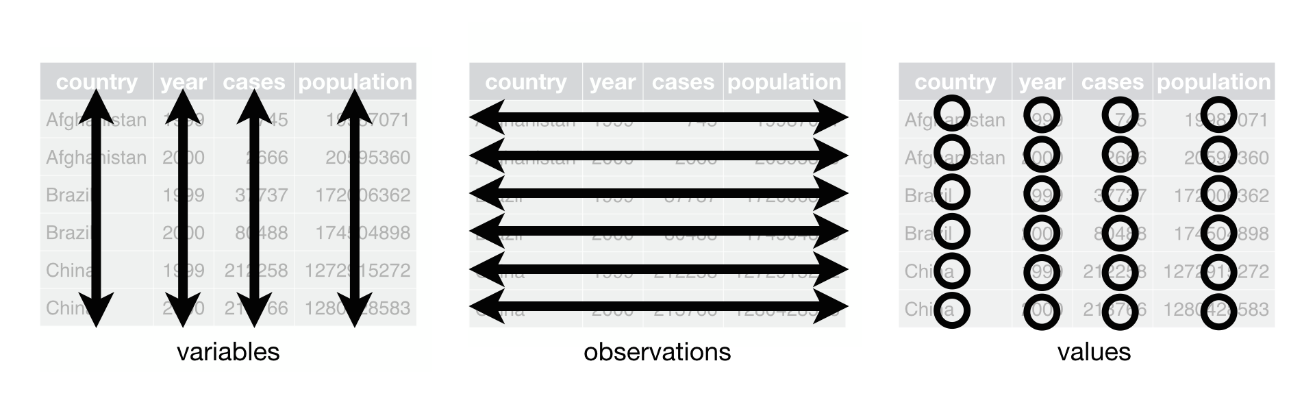
When the data is organized in a way where each column corresponds to a variable and each row corresponds to a observation, we consider the dataset tidy.
This image from Hadley Wickham’s excellent book R for Data Science visualizes the idea:
The name “tidy data” comes from Wickham’s paper (2014), that describes the ideas in great detail.
The choice of this data format is by no means a one man show: in fact Wickham cites Wes McKinney’s paper (2010) on Pandas’ chosen data format as an example of a tidy data format. In fact both R and Pandas developers recommend using tidy data.
Main reasons why this data format is recommended are:
It is easy to understand and helps to internalize how your data is organized.
In tidy data format all observations in a variable have the same data type. This means that columns can be stored as vectors. This saves memory and allows for vectorized calculations that are much faster.
It is easy for developers to create methods as they can assume how the data is organized.
There are cases where tidy data might not be the optimal format. For example, if your problem has matrices, you would not want to store it as rows and columns, but as a two-dimensional array. Another situation might arise when your data is in some other binary format e.g. image data. But in these cases you might want to use tidy data to store e.g. image names or model parameters.
In this course our data is mostly in tidy format and if it’s not in that format, we’ll want to convert our raw data into it as soon as possible.
Parsing Premiere League games - Problem 1
The exercise is provided in X_exercises/ch2-X-ex1.ipynb.
In the exercise we’ll create input parsing functions for Premier League results.
Look at the one of the
./data/england-master/XXXXs/XXXX-XX/eng.1.csv-datasets.Determine whether the data is in a tidy format.
If not, how would you modify the data format?
Simple data operations
Loading data from CSVs
Let’s start with loading data in the most common data format: csv. Quite often datasets are provided in this format because it is human readable and easy to transfer among systems.
Let’s consider a atp_players.csv-dataset that contains ATP ranks of men’s
singles tennis players.
Let’s load the data with the read_csv-function:
atp_players = pd.read_csv('../data/atp_players.csv', names=['player_id', 'first_name', 'last_name', 'hand', 'birth_date', 'country_code'])
atp_players.head()
        player_id       first_name      last_name       hand    birth_date      country_code
0       100001  Gardnar         Mulloy  R       19131122.0      USA
1       100002  Pancho  Segura  R       19210620.0      ECU
2       100003  Frank   Sedgman         R       19271002.0      AUS
3       100004  Giuseppe        Merlo   R       19271011.0      ITA
4       100005  Richard Pancho  Gonzales        R       19280509.0      USA
atp_players <- read_csv('../data/atp_players.csv', col_names=c('player_id', 'first_name', 'last_name', 'hand', 'birth_date', 'country_code'))
Parsed with column specification:
cols(
  player_id = col_double(),
  first_name = col_character(),
  last_name = col_character(),
  hand = col_character(),
  birth_date = col_double(),
  country_code = col_character()
)
player_id       first_name      last_name       hand    birth_date      country_code
100001  Gardnar         Mulloy  R       19131122        USA
100002  Pancho  Segura  R       19210620        ECU
100003  Frank   Sedgman         R       19271002        AUS
100004  Giuseppe        Merlo   R       19271011        ITA
100005  Richard Pancho  Gonzales        R       19280509        USA
100006  Grant   Golden  R       19290821        USA
This function not only parses the text, but also tries to convert the columns to a best possible fata types. To check column data types, use:
print(iris.dtypes)
player_id         int64
first_name       object
last_name        object
hand             object
birth_date      float64
country_code     object
dtype: object
str(atp_players)

Classes ‘spec_tbl_df’, ‘tbl_df’, ‘tbl’ and 'data.frame':        54938 obs. of  6 variables:
 $ player_id   : num  1e+05 1e+05 1e+05 1e+05 1e+05 ...
 $ first_name  : chr  "Gardnar" "Pancho" "Frank" "Giuseppe" ...
 $ last_name   : chr  "Mulloy" "Segura" "Sedgman" "Merlo" ...
 $ hand        : chr  "R" "R" "R" "R" ...
 $ birth_date  : num  19131122 19210620 19271002 19271011 19280509 ...
 $ country_code: chr  "USA" "ECU" "AUS" "ITA" ...
 - attr(*, "spec")=
  .. cols(
  ..   player_id = col_double(),
  ..   first_name = col_character(),
  ..   last_name = col_character(),
  ..   hand = col_character(),
  ..   birth_date = col_double(),
  ..   country_code = col_character()
  .. )
The head-function can be used to show the first few rows of our dataset.
atp_players.head()

        player_id       first_name      last_name       hand    birth_date      country_code
0       100001  Gardnar         Mulloy  R       19131122.0      USA
1       100002  Pancho  Segura  R       19210620.0      ECU
2       100003  Frank   Sedgman         R       19271002.0      AUS
3       100004  Giuseppe        Merlo   R       19271011.0      ITA
4       100005  Richard Pancho  Gonzales        R       19280509.0      USA
head(atp_players)

player_id       first_name      last_name       hand    birth_date      country_code
100001  Gardnar         Mulloy  R       19131122        USA
100002  Pancho  Segura  R       19210620        ECU
100003  Frank   Sedgman         R       19271002        AUS
100004  Giuseppe        Merlo   R       19271011        ITA
100005  Richard Pancho  Gonzales        R       19280509        USA
100006  Grant   Golden  R       19290821        USA
Creating and removing columns
Let’s start by converting the birth date column into an actual time stamp.
atp_players['birth_date'] = pd.to_datetime(atp_players['birth_date'], format='%Y%m%d', errors='coerce')
print(atp_players.dtypes)

player_id                int64
first_name              object
last_name               object
hand                    object
birth_date      datetime64[ns]
country_code            object
dtype: object
atp_players <- atp_players %>%
    mutate(birth_date=parse_date_time(birth_date, order='%Y%m%d'))
str(atp_players)

Warning message:
“ 125 failed to parse.”

Classes ‘spec_tbl_df’, ‘tbl_df’, ‘tbl’ and 'data.frame':        54938 obs. of  6 variables:
 $ player_id   : num  1e+05 1e+05 1e+05 1e+05 1e+05 ...
 $ first_name  : chr  "Gardnar" "Pancho" "Frank" "Giuseppe" ...
 $ last_name   : chr  "Mulloy" "Segura" "Sedgman" "Merlo" ...
 $ hand        : chr  "R" "R" "R" "R" ...
 $ birth_date  : POSIXct, format: "1913-11-22" "1921-06-20" ...
 $ country_code: chr  "USA" "ECU" "AUS" "ITA" ...
In our current situation we have separate columns for first and last names.
Let’s join these columns into one column called name:
atp_players['name'] = atp_players['last_name'] + ', ' + atp_players['first_name']

atp_players.head()

        player_id       first_name      last_name       hand    birth_date      country_code    name
0       100001  Gardnar         Mulloy  R       19131122.0      USA     Mulloy, Gardnar
1       100002  Pancho  Segura  R       19210620.0      ECU     Segura, Pancho
2       100003  Frank   Sedgman         R       19271002.0      AUS     Sedgman, Frank
3       100004  Giuseppe        Merlo   R       19271011.0      ITA     Merlo, Giuseppe
4       100005  Richard Pancho  Gonzales        R       19280509.0      USA     Gonzales, Richard Pancho
atp_players <- atp_players %>%
    unite(name, last_name, first_name, sep=', ', remove=FALSE)

head(atp_players)

player_id       name    first_name      last_name       hand    birth_date      country_code
100001  Mulloy, Gardnar         Gardnar         Mulloy  R       19131122        USA
100002  Segura, Pancho  Pancho  Segura  R       19210620        ECU
100003  Sedgman, Frank  Frank   Sedgman         R       19271002        AUS
100004  Merlo, Giuseppe         Giuseppe        Merlo   R       19271011        ITA
100005  Gonzales, Richard Pancho        Richard Pancho  Gonzales        R       19280509        USA
100006  Golden, Grant   Grant   Golden  R       19290821        USA
Now we can drop our unneeded columns:
atp_players.drop(['first_name','last_name'], axis=1, inplace=True)
atp_players.dtypes

player_id         int64
hand             object
birth_date      float64
country_code     object
name             object
dtype: object
atp_players <- atp_players %>%
    select(-first_name, -last_name)

str(atp_players)

Classes ‘tbl_df’, ‘tbl’ and 'data.frame':       54938 obs. of  5 variables:
 $ player_id   : num  1e+05 1e+05 1e+05 1e+05 1e+05 ...
 $ name        : chr  "Mulloy, Gardnar" "Segura, Pancho" "Sedgman, Frank" "Merlo, Giuseppe" ...
 $ hand        : chr  "R" "R" "R" "R" ...
 $ birth_date  : num  19131122 19210620 19271002 19271011 19280509 ...
 $ country_code: chr  "USA" "ECU" "AUS" "ITA" ...
Turning input processing tasks into functions
Now that we have an idea what operations we want to accomplish for our data loading, we should codify these operations by creating a data loading function.
Let’s create a data loading function for loading ATP player data:
def load_atp_players(atp_players_file):
    atp_players = pd.read_csv(atp_players_file, names=['player_id', 'first_name', 'last_name', 'hand', 'birth_date', 'country_code'])
    atp_players.loc[:,'birth_date'] = pd.to_datetime(atp_players.loc[:,'birth_date'], format='%Y%m%d', errors='coerce')
    atp_players['name'] = atp_players.loc[:,'last_name'] + ', ' + atp_players.loc[:,'first_name']
    atp_players.drop(['first_name','last_name'], axis=1, inplace=True)
    return atp_players

atp_players = load_atp_players('../data/atp_players.csv')
atp_players.head()

player_id       first_name      last_name       hand    birth_date      country_code    name
0       100001  Gardnar         Mulloy  R       1913-11-22      USA     Mulloy, Gardnar
1       100002  Pancho  Segura  R       1921-06-20      ECU     Segura, Pancho
2       100003  Frank   Sedgman         R       1927-10-02      AUS     Sedgman, Frank
3       100004  Giuseppe        Merlo   R       1927-10-11      ITA     Merlo, Giuseppe
4       100005  Richard Pancho  Gonzales        R       1928-05-09      USA     Gonzales, Richard Pancho
load_atp_players <- function(atp_players_file){
    atp_players <- read_csv(atp_players_file, col_names=c('player_id', 'first_name', 'last_name', 'hand', 'birth_date', 'country_code'), col_types=cols()) %>%
        mutate(birth_date=parse_date_time(birth_date, order='%Y%m%d')) %>%
        unite(name, last_name, first_name, sep=', ', remove=TRUE) %>%
        mutate_at(c('country_code', 'hand'), as.factor)
    return(atp_players)
}

atp_players <- load_atp_players('../data/atp_players.csv')
head(atp_players)

Warning message:
“ 125 failed to parse.”

player_id       name    hand    birth_date      country_code
100001  Mulloy, Gardnar         R       1913-11-22      USA
100002  Segura, Pancho  R       1921-06-20      ECU
100003  Sedgman, Frank  R       1927-10-02      AUS
100004  Merlo, Giuseppe         R       1927-10-11      ITA
100005  Gonzales, Richard Pancho        R       1928-05-09      USA
100006  Golden, Grant   R       1929-08-21      USA
Parsing Premiere League games - Problem 2
The exercise is provided in X_exercises/ch2-X-ex1.ipynb.
In this exercise we’ll create input parsing functions for Premier League results.
Create a function that loads the match data, converts date into a proper date object and determines the season from the date.
Categorical data format
When working with string data that has well defined categories, it is usually a good idea to convert the data into categorical (Python) / factor (R) format. In this format all unique strings are given an integer value and the string array is converted into an integer array with this mapping. The unique strings are called “categories” or “levels” of the categorical/factor array.
Main benefits of using categorical data are:
Makes it easier to re-categorize the data by combining levels.
Helps with grouping and plot labeling.
Reduced memory consumption.
Disadvantages include:
For string arrays with completely unique values (e.g. our
name-column), most of the benefits are lost.Some models may recognize categorical data as numeric data as the underlying format in memory is an integer array. Check documentation of your modeling function whether it works with categorical data.
atp_players_categorized = atp_players.copy()
print(atp_players_categorized['hand'].nbytes)
atp_players_categorized.loc[:,['country_code', 'hand']] = atp_players_categorized.loc[:, ['country_code', 'hand']].apply(lambda x: x.astype('category'))
print(atp_players_categorized['country_code'].nbytes)
print(atp_players_categorized['hand'].cat.categories)
atp_players_categorized.dtypes

54970
111556
Index(['A', 'L', 'R', 'U'], dtype='object')

player_id                int64
hand                  category
birth_date      datetime64[ns]
country_code          category
name                    object
dtype: object
object.size(atp_players[['hand']])
atp_players <- atp_players %>%
    mutate_at(c('country_code', 'hand'), as.factor)
object.size(atp_players[['hand']])
print(levels(atp_players[['hand']]))
str(atp_players)

439776 bytes
220440 bytes
[1] "A" "L" "R" "U"
Classes ‘tbl_df’, ‘tbl’ and 'data.frame':       54938 obs. of  5 variables:
 $ player_id   : num  1e+05 1e+05 1e+05 1e+05 1e+05 ...
 $ name        : chr  "Mulloy, Gardnar" "Segura, Pancho" "Sedgman, Frank" "Merlo, Giuseppe" ...
 $ hand        : Factor w/ 4 levels "A","L","R","U": 3 3 3 3 3 3 2 3 3 3 ...
 $ birth_date  : num  19131122 19210620 19271002 19271011 19280509 ...
 $ country_code: Factor w/ 210 levels "AFG","AHO","ALB",..: 200 62 13 97 200 200 160 58 88 43 ...
Let’s create a function for this behaviour as well:
def categorize_players(players):
    players.loc[:,['country_code', 'hand']] = players.loc[:, ['country_code', 'hand']].apply(lambda x: x.astype('category'))
    return players

print(atp_players.dtypes)
atp_players = categorize_players(atp_players)
atp_players.dtypes

player_id                int64
hand                    object
birth_date      datetime64[ns]
country_code            object
name                    object
dtype: object

player_id                int64
hand                  category
birth_date      datetime64[ns]
country_code          category
name                    object
dtype: object
categorize_players <- function(players) {
    players <- players %>%
        mutate_at(c('country_code', 'hand'), as.factor)
    return(players)
}
str(atp_players)
atp_players <- categorize_players(atp_players)
str(atp_players)

Classes ‘tbl_df’, ‘tbl’ and 'data.frame':       54938 obs. of  5 variables:
 $ player_id   : num  1e+05 1e+05 1e+05 1e+05 1e+05 ...
 $ name        : chr  "Mulloy, Gardnar" "Segura, Pancho" "Sedgman, Frank" "Merlo, Giuseppe" ...
 $ hand        : chr  "R" "R" "R" "R" ...
 $ birth_date  : POSIXct, format: "1913-11-22" "1921-06-20" ...
 $ country_code: chr  "USA" "ECU" "AUS" "ITA" ...
Classes ‘tbl_df’, ‘tbl’ and 'data.frame':       54938 obs. of  5 variables:
 $ player_id   : num  1e+05 1e+05 1e+05 1e+05 1e+05 ...
 $ name        : chr  "Mulloy, Gardnar" "Segura, Pancho" "Sedgman, Frank" "Merlo, Giuseppe" ...
 $ hand        : Factor w/ 4 levels "A","L","R","U": 3 3 3 3 3 3 2 3 3 3 ...
 $ birth_date  : POSIXct, format: "1913-11-22" "1921-06-20" ...
 $ country_code: Factor w/ 210 levels "AFG","AHO","ALB",..: 200 62 13 97 200 200 160 58 88 43 ...
Joining datasets together
Quite often the data one obtains is not in a single file, but spread across multiple files. In situations like these you’ll need to combine these datasets. However, there are different ways to combine datasets:
Concatenation / adding rows. In concatenation one dataset, with a certain column format, is combined with another dataset with the same column format. This process is usually slow because adding rows requires allocation of new column vectors. Thus one should avoid these operations beyond the initial data creation.
Joining / adding columns. During joining process columns from a dataset with a certain column format are added into another dataset with a different column format. When joining, it is important that the datasets have a some common column (or an index) that can be used to match different rows/observations. This process is usually fast, but one should always determine the correct type of join type (left, right, union, full) to avoid unnecessary NA-values. With large datasets (or databases) one should also always first select the areas of interest and join those, not the other way around.
Let’s consider the data files atp_rankings_00s.csv and
atp_rankings_10s.csv that contain the weekly ATP rankings from the
2000s and 2010s. Let’s load these datasets:
def load_atp_rankings(atp_rankings_file):
    atp_rankings = pd.read_csv(atp_rankings_file)
    atp_rankings.loc[:,'ranking_date'] = pd.to_datetime(atp_rankings.loc[:, 'ranking_date'], format='%Y%m%d', errors='coerce')
    return atp_rankings

atp_rankings00 = load_atp_rankings('../data/atp_rankings_00s.csv')
atp_rankings10 = load_atp_rankings('../data/atp_rankings_10s.csv')

print(atp_rankings00.head())
print(atp_rankings10.head())

  ranking_date  rank  player  points
0   2000-01-10     1  101736  4135.0
1   2000-01-10     2  102338  2915.0
2   2000-01-10     3  101948  2419.0
3   2000-01-10     4  103017  2184.0
4   2000-01-10     5  102856  2169.0
  ranking_date  rank  player   points
0   2010-01-04     1  103819  10550.0
1   2010-01-04     2  104745   9205.0
2   2010-01-04     3  104925   8310.0
3   2010-01-04     4  104918   7030.0
4   2010-01-04     5  105223   6785.0
load_atp_rankings <- function(atp_rankings_file){
    atp_rankings <- read_csv(atp_rankings_file, col_types=cols()) %>%
        mutate(ranking_date=parse_date_time(ranking_date, order='%Y%m%d'))
    return(atp_rankings)
}

atp_rankings00 <- load_atp_rankings('../data/atp_rankings_00s.csv')
atp_rankings10 <- load_atp_rankings('../data/atp_rankings_10s.csv')

head(atp_rankings00)
head(atp_rankings10)

ranking_date    rank    player  points
2000-01-10      1       101736  4135
2000-01-10      2       102338  2915
2000-01-10      3       101948  2419
2000-01-10      4       103017  2184
2000-01-10      5       102856  2169
2000-01-10      6       102358  2107
ranking_date    rank    player  points
2010-01-04      1       103819  10550
2010-01-04      2       104745  9205
2010-01-04      3       104925  8310
2010-01-04      4       104918  7030
2010-01-04      5       105223  6785
2010-01-04      6       103786  4930
Now, as we have two datasets with identical column format, we’ll want to concatenate these datasets together:
print(atp_rankings00.shape)
print(atp_rankings10.shape)
atp_rankings = pd.concat([atp_rankings00, atp_rankings10], ignore_index=True)
print(atp_rankings.shape)
atp_rankings.head()

(920907, 4)
(916296, 4)
(1837203, 4)

    ranking_date        rank    player  points
0       2000-01-10      1       101736  4135.0
1       2000-01-10      2       102338  2915.0
2       2000-01-10      3       101948  2419.0
3       2000-01-10      4       103017  2184.0
4       2000-01-10      5       102856  2169.0
print(nrow(atp_rankings00))
print(nrow(atp_rankings10))
atp_rankings <- bind_rows(atp_rankings00, atp_rankings10)
print(nrow(atp_rankings))
print(head(atp_rankings))

[1] 920907
[1] 916296
[1] 1837203
# A tibble: 6 x 4
  ranking_date         rank player points
  <dttm>              <dbl>  <dbl>  <dbl>
1 2000-01-10 00:00:00     1 101736   4135
2 2000-01-10 00:00:00     2 102338   2915
3 2000-01-10 00:00:00     3 101948   2419
4 2000-01-10 00:00:00     4 103017   2184
5 2000-01-10 00:00:00     5 102856   2169
6 2000-01-10 00:00:00     6 102358   2107
At this point we can notice that the player identification number is not the same on player- and ranking-datasets. We should rename this column, as we will be using that to join these datasets together.
atp_rankings.rename(columns={'player':'player_id'}, inplace=True)

atp_rankings.head()

    ranking_date        rank    player_id       points
0       2000-01-10      1       101736  4135.0
1       2000-01-10      2       102338  2915.0
2       2000-01-10      3       101948  2419.0
3       2000-01-10      4       103017  2184.0
4       2000-01-10      5       102856  2169.0
atp_rankings <- atp_rankings %>%

    rename(player_id=player)

head(atp_rankings)

ranking_date    rank    player_id       points
2000-01-10      1       101736  4135
2000-01-10      2       102338  2915
2000-01-10      3       101948  2419
2000-01-10      4       103017  2184
2000-01-10      5       102856  2169
2000-01-10      6       102358  2107
Now that we have figured how we want to parse these datasets, let’s create a function that can read multiple files with a for-loop structure.
def load_multiple_atp_rankings(atp_rankings_files):
    datasets = []
    for atp_ranking_file in atp_rankings_files:
        dataset = load_atp_rankings(atp_ranking_file)
        datasets.append(dataset)
    atp_rankings = pd.concat(datasets, ignore_index=True)
    atp_rankings.rename(columns={'player':'player_id'}, inplace=True)
    return atp_rankings

atp_rankings = load_multiple_atp_rankings(['../data/atp_rankings_00s.csv','../data/atp_rankings_10s.csv'])
print(atp_rankings.shape)
atp_rankings.head()

(1837203, 4)

    ranking_date        rank    player_id       points
0       2000-01-10      1       101736  4135.0
1       2000-01-10      2       102338  2915.0
2       2000-01-10      3       101948  2419.0
3       2000-01-10      4       103017  2184.0
4       2000-01-10      5       102856  2169.0
load_multiple_atp_rankings <- function(atp_rankings_files){
    datasets <- list()
    for (atp_ranking_file in atp_rankings_files) {
        dataset <- load_atp_rankings(atp_ranking_file)
        datasets <- append(datasets, list(dataset))
    }
    atp_rankings <- bind_rows(datasets) %>%
        rename(player_id=player)
    return(atp_rankings)
}

atp_rankings <- load_multiple_atp_rankings(c('../data/atp_rankings_00s.csv','../data/atp_rankings_10s.csv'))
print(nrow(atp_rankings))
head(atp_rankings)

[1] 1837203

ranking_date    rank    player_id       points
2000-01-10      1       101736  4135
2000-01-10      2       102338  2915
2000-01-10      3       101948  2419
2000-01-10      4       103017  2184
2000-01-10      5       102856  2169
2000-01-10      6       102358  2107
This new function provides an interesting feature: we do not need to create duplicate variables for our new datasets. We could be reading 2 or 2000 files and our function would work identically.
Let’s now combine this rankings dataset with our player dataset. Now we’re
going to do dataset joining with player_id as our joining column. As our
players dataset contains a lot of players who did not play during the time
period that we have in our rankings dataset, we should use the rankings
dataset as our master dataset and do a left join. This means that we only
join those rows from the players dataset that have corresponding player ID
in our rankings dataset.
atp_data = atp_rankings.merge(atp_players, on='player_id', how='left')
print(atp_data.dtypes)
atp_data.head()

ranking_date    datetime64[ns]
rank                     int64
player_id                int64
points                 float64
hand                  category
birth_date      datetime64[ns]
country_code          category
name                    object
dtype: object

    ranking_date        rank    player_id       points  hand    birth_date      country_code    name
0       2000-01-10      1       101736  4135.0  R       1970-04-29      USA     Agassi, Andre
1       2000-01-10      2       102338  2915.0  R       1974-02-18      RUS     Kafelnikov, Yevgeny
2       2000-01-10      3       101948  2419.0  R       1971-08-12      USA     Sampras, Pete
3       2000-01-10      4       103017  2184.0  R       1977-07-05      GER     Kiefer, Nicolas
4       2000-01-10      5       102856  2169.0  R       1976-09-10      BRA     Kuerten, Gustavo
atp_data <- atp_rankings %>%
    left_join(atp_players, by='player_id')
str(atp_data)
head(atp_data)

Classes ‘spec_tbl_df’, ‘tbl_df’, ‘tbl’ and 'data.frame':        1837203 obs. of  8 variables:
 $ ranking_date: POSIXct, format: "2000-01-10" "2000-01-10" ...
 $ rank        : num  1 2 3 4 5 6 7 8 9 10 ...
 $ player_id   : num  101736 102338 101948 103017 102856 ...
 $ points      : num  4135 2915 2419 2184 2169 ...
 $ name        : chr  "Agassi, Andre" "Kafelnikov, Yevgeny" "Sampras, Pete" "Kiefer, Nicolas" ...
 $ hand        : Factor w/ 4 levels "A","L","R","U": 3 3 3 3 3 3 3 3 2 3 ...
 $ birth_date  : POSIXct, format: "1970-04-29" "1974-02-18" ...
 $ country_code: Factor w/ 210 levels "AFG","AHO","ALB",..: 200 161 200 76 28 179 62 200 43 137 ...

ranking_date    rank    player_id       points  name    hand    birth_date      country_code
2000-01-10      1       101736  4135    Agassi, Andre   R       1970-04-29      USA
2000-01-10      2       102338  2915    Kafelnikov, Yevgeny     R       1974-02-18      RUS
2000-01-10      3       101948  2419    Sampras, Pete   R       1971-08-12      USA
2000-01-10      4       103017  2184    Kiefer, Nicolas         R       1977-07-05      GER
2000-01-10      5       102856  2169    Kuerten, Gustavo        R       1976-09-10      BRA
2000-01-10      6       102358  2107    Enqvist, Thomas         R       1974-03-13      SWE
Parsing Premiere League games - Problems 3, 4 and 5
The exercise is provided in X_exercises/ch2-X-ex1.ipynb.
In this exercise we’ll create input parsing functions for Premier League results.
Problems 3, 4 and 5:
Create a function that formats the data into a tidy format and adds additional information based on existing data.
Create a function that turns some of our columns into categorical format.
Create a function that can combine multiple data files into a single dataset.
After solving problem 2 and 3 you can try out two demonstrations of what can be done with the data:
Check whether home side has an advantage in football games.
Calculate Premier League winners.
Demonstrating ATP dataset: Longest reign at rank 1
Let’s use our newly generated dataset to find out who has had the longest reign at top 1 spot during this time period. Now we’re only interested on players that have attained rank 1. Let’s pick only those rows.
atp_top1 = atp_data.loc[atp_data.loc[:,'rank']==1].copy()
atp_top1.head()

    ranking_date        rank    player_id       points  hand    birth_date      country_code    name
0       2000-01-10      1       101736  4135.0  R       1970-04-29      USA     Agassi, Andre
1572    2000-01-17      1       101736  4135.0  R       1970-04-29      USA     Agassi, Andre
3143    2000-01-24      1       101736  4135.0  R       1970-04-29      USA     Agassi, Andre
4713    2000-01-31      1       101736  5045.0  R       1970-04-29      USA     Agassi, Andre
6287    2000-02-07      1       101736  5045.0  R       1970-04-29      USA     Agassi, Andre
# Better when we want to drop rows
atp_top1 <- atp_data %>%
    filter(rank == 1)

# or

# Logical indexing is more useful when we want to edit certain rows
atp_top1 <- atp_data[atp_data['rank'] == 1,]

head(atp_top1)

 ranking_date   rank    player_id       points  name    hand    birth_date      country_code
2000-01-10      1       101736  4135    Agassi, Andre   R       1970-04-29      USA
2000-01-17      1       101736  4135    Agassi, Andre   R       1970-04-29      USA
2000-01-24      1       101736  4135    Agassi, Andre   R       1970-04-29      USA
2000-01-31      1       101736  5045    Agassi, Andre   R       1970-04-29      USA
2000-02-07      1       101736  5045    Agassi, Andre   R       1970-04-29      USA
2000-02-14      1       101736  5045    Agassi, Andre   R       1970-04-29      USA
In order to see when the top 1 rank holder has changed we’ll create a new
column previous_top that contains a shifted version of the player name.
atp_top1.loc[:, 'previous_top'] = atp_top1['player_id'].shift(1)
atp_top1.head()

ranking_date    rank    player_id       points  hand    birth_date      country_code    name    previous_top
0       2000-01-10      1       101736  4135.0  R       1970-04-29      USA     Agassi, Andre   NaN
1572    2000-01-17      1       101736  4135.0  R       1970-04-29      USA     Agassi, Andre   101736.0
3143    2000-01-24      1       101736  4135.0  R       1970-04-29      USA     Agassi, Andre   101736.0
4713    2000-01-31      1       101736  5045.0  R       1970-04-29      USA     Agassi, Andre   101736.0
6287    2000-02-07      1       101736  5045.0  R       1970-04-29      USA     Agassi, Andre   101736.0
atp_top1 <- atp_top1 %>%
    mutate(previous_top=lag(player_id))

head(atp_top1)

ranking_date    rank    player_id       points  name    hand    birth_date      country_code    previous_top
2000-01-10      1       101736  4135    Agassi, Andre   R       1970-04-29      USA     NA
2000-01-17      1       101736  4135    Agassi, Andre   R       1970-04-29      USA     101736
2000-01-24      1       101736  4135    Agassi, Andre   R       1970-04-29      USA     101736
2000-01-31      1       101736  5045    Agassi, Andre   R       1970-04-29      USA     101736
2000-02-07      1       101736  5045    Agassi, Andre   R       1970-04-29      USA     101736
2000-02-14      1       101736  5045    Agassi, Andre   R       1970-04-29      USA     101736
Now let’s further limit ourselves to those observations where the reign has changed. That is, rank 1 player is different to previous player.
atp_top1_reigns = atp_top1.loc[atp_top1['player_id'] != atp_top1['previous_top'],:].copy()
atp_top1_reigns.head()

ranking_date    rank    player_id       points  hand    birth_date      country_code    name    previous_top
0       2000-01-10      1       101736  4135.0  R       1970-04-29      USA     Agassi, Andre   NaN
55359   2000-09-11      1       101948  3739.0  R       1971-08-12      USA     Sampras, Pete   101736.0
71523   2000-11-20      1       103498  3920.0  R       1980-01-27      RUS     Safin, Marat    101948.0
74761   2000-12-04      1       102856  4195.0  R       1976-09-10      BRA     Kuerten, Gustavo        103498.0
87617   2001-01-29      1       103498  4265.0  R       1980-01-27      RUS     Safin, Marat    102856.0
# Better when we want to drop rows
atp_top1_reigns <- atp_top1 %>%
    filter(player_id != previous_top)
head(atp_top1_reigns)

# Logical indexing is more useful when we want to edit certain rows
atp_top1_reigns <- drop_na(atp_top1[atp_top1['player_id'] != atp_top1['previous_top'],])
head(atp_top1_reigns)

 ranking_date   rank    player_id       points  name    hand    birth_date      country_code    previous_top
2000-09-11      1       101948  3739    Sampras, Pete   R       1971-08-12      USA     101736
2000-11-20      1       103498  3920    Safin, Marat    R       1980-01-27      RUS     101948
2000-12-04      1       102856  4195    Kuerten, Gustavo        R       1976-09-10      BRA     103498
2001-01-29      1       103498  4265    Safin, Marat    R       1980-01-27      RUS     102856
2001-02-26      1       102856  4365    Kuerten, Gustavo        R       1976-09-10      BRA     103498
2001-04-02      1       103498  4270    Safin, Marat    R       1980-01-27      RUS     102856
Now we’ll want to calculate the reign lengths of our top 1 players. To do this we’ll calculate the difference on our ranking dates and shift it so that the result matches the player.
atp_top1_reigns['reign_length'] = atp_top1_reigns.loc[:,'ranking_date'].diff().shift(-1)
atp_top1_reigns.head()

ranking_date    rank    player_id       points  hand    birth_date      country_code    name    previous_top    reign_length
0       2000-01-10      1       101736  4135.0  R       1970-04-29      USA     Agassi, Andre           NaN             245 days
55359   2000-09-11      1       101948  3739.0  R       1971-08-12      USA     Sampras, Pete           101736.0        70 days
71523   2000-11-20      1       103498  3920.0  R       1980-01-27      RUS     Safin, Marat            101948.0        14 days
74761   2000-12-04      1       102856  4195.0  R       1976-09-10      BRA     Kuerten, Gustavo        103498.0        56 days
87617   2001-01-29      1       103498  4265.0  R       1980-01-27      RUS     Safin, Marat            102856.0        28 days
atp_top1_reigns <- atp_top1_reigns %>%
    mutate(reign_length=difftime(lead(ranking_date), ranking_date))
head(atp_top1_reigns)

ranking_date    rank    player_id       points  name    hand    birth_date      country_code    previous_top    reign_length
2000-09-11      1       101948  3739    Sampras, Pete   R       1971-08-12      USA     101736  70 days
2000-11-20      1       103498  3920    Safin, Marat    R       1980-01-27      RUS     101948  14 days
2000-12-04      1       102856  4195    Kuerten, Gustavo        R       1976-09-10      BRA     103498  56 days
2001-01-29      1       103498  4265    Safin, Marat    R       1980-01-27      RUS     102856  28 days
2001-02-26      1       102856  4365    Kuerten, Gustavo        R       1976-09-10      BRA     103498  35 days
2001-04-02      1       103498  4270    Safin, Marat    R       1980-01-27      RUS     102856  21 days
Now let’s sort these values to obtain the longest reigns. When we compare the results with this list of top reigns, we see that we have captured many of these reigns in our dataset.
atp_top1_reigns.sort_values('reign_length', ascending=False).head(5)

ranking_date    rank    player_id       points  hand    birth_date      country_code    name    previous_top    reign_length
346974          2004-02-02      1       103819  5225.0          R       1981-08-08      SUI     Federer, Roger          104053.0        1659 days
1331200         2014-07-07      1       104925  13130.0         R       1987-05-22      SRB     Djokovic, Novak         104745.0        854 days
155503          2001-11-19      1       103720  4365.0          R       1981-02-24      AUS     Hewitt, Lleyton         102856.0        525 days
960449          2010-06-07      1       104745  8700.0          L       1986-06-03      ESP     Nadal, Rafael           103819.0        392 days
1050927         2011-07-04      1       104925  13285.0         R       1987-05-22      SRB     Djokovic, Novak         104745.0        371 days
atp_top1_reigns %>%
    top_n(5, reign_length) %>%
    arrange(desc(reign_length))

 ranking_date   rank    player_id       points  name    hand    birth_date      country_code    previous_top    reign_length
2004-02-02      1       103819  5225    Federer, Roger  R       1981-08-08      SUI     104053  1659 days
2014-07-07      1       104925  13130   Djokovic, Novak R       1987-05-22      SRB     104745  854 days
2001-11-19      1       103720  4365    Hewitt, Lleyton R       1981-02-24      AUS     102856  525 days
2010-06-07      1       104745  8700    Nadal, Rafael   L       1986-06-03      ESP     103819  392 days
2011-07-04      1       104925  13285   Djokovic, Novak R       1987-05-22      SRB     104745  371 days
Using binary data formats to improve your pipeline
Why binary data formats?
Quite often raw data is provided as CSVs or other delimited files (e.g.
.dat-files). Sometimes you have a zips that contain huge amount of
individual files or images. Reading such files can be slow, resource intensive,
bad for a shared file system and complicated as one needs to do parsing each
time the files are loaded.
In situations like it is usually a good idea to do basic parsing for the data and store a working copy of the data in a binary format. Even though this causes data duplication, the performance benefits will easily outweight this cost. Benefits of binary formats include:
Data size is reduced due to better encodings (e.g. ASCII vs. binary float).
Data loading is much faster due to reduced parsing and better buffering behavior.
All of the data does not need to be loaded in order to access parts of the data.
Raw data can be stored in a separate location which reduces the risk of spoiling the raw data.
One should take few things into account when using binary data formats:
Choose a binary format that best suits the problem at hand. There isn’t one data format that works in all cases.
Write the files programatically using pipeline functions. This makes testing easier and allows others to replicate your data format from the raw data.
If the format supports metadata attributes, use them to store e.g. code revision used to create the dataset, hyperparameters of the model used etc.
Of course one should also use binary data formats to store temporary data or intermediate results from the models. Easily readable/transferable formats such as CSVs can be used when the results are being shared and datasets are published, but due to reasons mentioned before, they are not optimal for storing temporary results.
CSVs
CSVs (and other delimited text files) are common, but they are rarely the best format to use throughout a pipeline. Raw datasets are often provided in CSV format as it is very easy to transport.
Pros:
CSVs are human readable, so data loading is easy to verify.
They area usually easy to parse.
Easy to share with other users.
Cons:
One usually needs to manually specify column names, column types, delimiters etc.
Data is stored very inefficiently. Storing e.g. a floating point number in ASCII takes a lot more space than storing it as binary.
Using bad data readers (e.g. reading file without read_csv-functions) can result in huge number of small IO operations as text reading usually reads file some 4-64 kB at a time (a.k.a. small buffer size).
read_csvdata loaders usually require lots of memory as data needs to be first loaded as generic strings before it can be parsed to binary columns.Reading huge CSV files requires using more advanced libraries like Dask (Python) or data.table (R).
There are many binary data formats that one can use to mitigate most of these issues. We’ll be looking at them next, but first let’s save our data as a CSV file using the writing functions.
atp_data.to_csv('../data/atp_data_python.csv')
pd.read_csv('../data/atp_data_python.csv').head()

Unnamed: 0      ranking_date    rank    player_id       points  hand    birth_date      country_code    name
0       0       2000-01-10      1       101736  4135.0  R       1970-04-29      USA     Agassi, Andre
1       1       2000-01-10      2       102338  2915.0  R       1974-02-18      RUS     Kafelnikov, Yevgeny
2       2       2000-01-10      3       101948  2419.0  R       1971-08-12      USA     Sampras, Pete
3       3       2000-01-10      4       103017  2184.0  R       1977-07-05      GER     Kiefer, Nicolas
4       4       2000-01-10      5       102856  2169.0  R       1976-09-10      BRA     Kuerten, Gustavo
write_csv(atp_data, '../data/atp_data_r.csv')
head(read_csv('../data/atp_data_r.csv'))

Parsed with column specification:
cols(
  ranking_date = col_datetime(format = ""),
  rank = col_double(),
  player_id = col_double(),
  points = col_double(),
  name = col_character(),
  hand = col_character(),
  birth_date = col_datetime(format = ""),
  country_code = col_character()
)

ranking_date    rank    player_id       points  name    hand    birth_date      country_code
2000-01-10      1       101736  4135    Agassi, Andre   R       1970-04-29      USA
2000-01-10      2       102338  2915    Kafelnikov, Yevgeny     R       1974-02-18      RUS
2000-01-10      3       101948  2419    Sampras, Pete   R       1971-08-12      USA
2000-01-10      4       103017  2184    Kiefer, Nicolas         R       1977-07-05      GER
2000-01-10      5       102856  2169    Kuerten, Gustavo        R       1976-09-10      BRA
2000-01-10      6       102358  2107    Enqvist, Thomas         R       1974-03-13      SWE
Serialized objects
Serialized objects are basically the objects stored into file as they are in memory. In Python the default serialized format is Pickle and in R Rdata.
Pros:
Easy to write and read.
Binary data format.
Data can be automatically compressed.
Cons:
Data needs to be read as is was. You cannot easily read only parts of it.
Somewhat unreliable to share.
Buffer size is most likely not very big.
Serialized objects are good for debugging the state of the code, but not necessarily best for actual data storage or transporting to collaborators. At the same time they support all kinds of objects, so they are good if you do not have a better format.
Let’s save our atp_data-dataset using these formats:
atp_data.to_pickle('../data/atp_data.pickle.gz')
pd.read_pickle('../data/atp_data.pickle.gz').head()

    ranking_date        rank    player_id       points  hand    birth_date      country_code    name
0       2000-01-10      1       101736  4135.0  R       1970-04-29      USA     Agassi, Andre
1       2000-01-10      2       102338  2915.0  R       1974-02-18      RUS     Kafelnikov, Yevgeny
2       2000-01-10      3       101948  2419.0  R       1971-08-12      USA     Sampras, Pete
3       2000-01-10      4       103017  2184.0  R       1977-07-05      GER     Kiefer, Nicolas
4       2000-01-10      5       102856  2169.0  R       1976-09-10      BRA     Kuerten, Gustavo
save(atp_data, file='../data/atp_data.Rdata')
rm(atp_data)

load('../data/atp_data.Rdata')
head(atp_data)

ranking_date    rank    player_id       points  name    hand    birth_date      country_code
2000-01-10      1       101736  4135    Agassi, Andre   R       1970-04-29      USA
2000-01-10      2       102338  2915    Kafelnikov, Yevgeny     R       1974-02-18      RUS
2000-01-10      3       101948  2419    Sampras, Pete   R       1971-08-12      USA
2000-01-10      4       103017  2184    Kiefer, Nicolas         R       1977-07-05      GER
2000-01-10      5       102856  2169    Kuerten, Gustavo        R       1976-09-10      BRA
2000-01-10      6       102358  2107    Enqvist, Thomas         R       1974-03-13      SWE
Feather
Important
The course environment.yml contains a older implementations
of the feather-format from feather-library.
Nowadays R has a faster feather in arrow-library.
Likewise Python implementation is nowadays included in
pyarrow-library,
and environment.yml installed the old version, which no longer works.
To install the newer versions, please run
conda install --freeze-installed -c conda-forge pyarrow=1.0.1 r-arrow=1.0.1 r-vctrs
in an Anaconda shell.
Please use the arrow-versions, if you want to use feather with your
own code.
Feather format is a data format for efficient storing of tabular data. It’s built on top of Apache Arrow columnar data specification and it was created by the developers of Pandas and Tidyverse to allow writing and reading big tables from both Pandas and R. Nowadays it’s development is deeply connected with the Apache Arrow format.
Pros:
Easy to write and read.
Very fast.
Good for columnar data.
Good format for moving columnar data between R and Python.
Cons:
Only for tabular data.
Limited amount of supported column data formats.
Not something for long term storage as the format is quite new.
Let’s save our atp_data-dataset using feather:
atp_data.to_feather('../data/atp_data_python.feather')
pd.read_feather('../data/atp_data_python.feather').head()

    ranking_date        rank    player_id       points  hand    birth_date      country_code    name
0       2000-01-10      1       101736  4135.0  R       1970-04-29      USA     Agassi, Andre
1       2000-01-10      2       102338  2915.0  R       1974-02-18      RUS     Kafelnikov, Yevgeny
2       2000-01-10      3       101948  2419.0  R       1971-08-12      USA     Sampras, Pete
3       2000-01-10      4       103017  2184.0  R       1977-07-05      GER     Kiefer, Nicolas
4       2000-01-10      5       102856  2169.0  R       1976-09-10      BRA     Kuerten, Gustavo
arrow’s write_feather arrow’s read_feather
library(arrow)
write_feather(atp_data ,'../data/atp_data_r.feather')
head(read_feather('../data/atp_data_r.feather'))

ranking_date    rank    player_id       points  name    hand    birth_date      country_code
2000-01-10      1       101736  4135    Agassi, Andre   R       1970-04-29      USA
2000-01-10      2       102338  2915    Kafelnikov, Yevgeny     R       1974-02-18      RUS
2000-01-10      3       101948  2419    Sampras, Pete   R       1971-08-12      USA
2000-01-10      4       103017  2184    Kiefer, Nicolas         R       1977-07-05      GER
2000-01-10      5       102856  2169    Kuerten, Gustavo        R       1976-09-10      BRA
2000-01-10      6       102358  2107    Enqvist, Thomas         R       1974-03-13      SWE
Parquet
Apache Parquet is a columnar data format that many big data systems use to store data in their backend. The format uses multiple levels of encoding and compression to reduce file size.
Pros:
Easy to write and read.
Very efficient spacewise.
Good for long-term storage.
Easy to read into big data applications (Spark/Hadoop/etc.)
Good interoperability between different languages.
Supports metadata in data files.
Cons:
Slower to read from / write to disk due to encoding and compression.
Big data access needs well designed workflows for efficient data loading.
Wes McKinney has made a good blog post about performance of Feather, Parquet and other popular formats.
pyarrow’s parquet-functionality
atp_data.to_parquet('../data/atp_data_python.parquet')
pd.read_parquet('../data/atp_data_python.parquet').head()

    ranking_date        rank    player_id       points  hand    birth_date      country_code    name
0       2000-01-10      1       101736  4135.0  R       1970-04-29      USA     Agassi, Andre
1       2000-01-10      2       102338  2915.0  R       1974-02-18      RUS     Kafelnikov, Yevgeny
2       2000-01-10      3       101948  2419.0  R       1971-08-12      USA     Sampras, Pete
3       2000-01-10      4       103017  2184.0  R       1977-07-05      GER     Kiefer, Nicolas
4       2000-01-10      5       102856  2169.0  R       1976-09-10      BRA     Kuerten, Gustavo
arrow-library’s write_parquet arrow-library’s read_parquet
library(arrow)
write_parquet(atp_data ,'../data/atp_data_r.parquet')
head(read_parquet('../data/atp_data_r.parquet'))

ranking_date    rank    player_id       points  name    hand    birth_date      country_code
2000-01-10      1       101736  4135    Agassi, Andre   R       1970-04-29      USA
2000-01-10      2       102338  2915    Kafelnikov, Yevgeny     R       1974-02-18      RUS
2000-01-10      3       101948  2419    Sampras, Pete   R       1971-08-12      USA
2000-01-10      4       103017  2184    Kiefer, Nicolas         R       1977-07-05      GER
2000-01-10      5       102856  2169    Kuerten, Gustavo        R       1976-09-10      BRA
2000-01-10      6       102358  2107    Enqvist, Thomas         R       1974-03-13      SWE
HDF5
Important
R interface to HDF was missing from environment.yml. If you want to
install it, please run
conda install --freeze-installed -c conda-forge r-hdf5r
in an Anaconda shell.
Hierarchical Data Format version 5 (HDF5) is a binary format designed to store multiple datasets in a single file. It is especially used to store array data in physics and similar fields with large arrays, but it can be used to store other data as well.
Pros:
Good for matrices or other big binary arrays.
Hierarchical data format where you can store multiple datasets and metadata in a single file.
Fast when reading big chunks.
Good for sharing finished datasets.
Cons:
Bad performance when you want to do random reads from within a dataset.
Similar directory management hassle as with individual files.
Pandas HDF5 interface uses pickled pytables-objects, so the format is no longer that good for sharing. h5py is a better interface for full access to all HDF features.
R interface is quite clunky.
atp_data.to_hdf('../data/atp_data_python.h5', '/atp_data', format='table')
pd.read_hdf('../data/atp_data_python.h5','/atp_data').head()

    ranking_date        rank    player_id       points  hand    birth_date      country_code    name
0       2000-01-10      1       101736  4135.0  R       1970-04-29      USA     Agassi, Andre
1       2000-01-10      2       102338  2915.0  R       1974-02-18      RUS     Kafelnikov, Yevgeny
2       2000-01-10      3       101948  2419.0  R       1971-08-12      USA     Sampras, Pete
3       2000-01-10      4       103017  2184.0  R       1977-07-05      GER     Kiefer, Nicolas
4       2000-01-10      5       102856  2169.0  R       1976-09-10      BRA     Kuerten, Gustavo
library(hdf5r)
h5_file <- H5File$new('../data/atp_data_r.h5', mode = 'w')
h5_group <- h5_file$create_group('atp_data')
for (column in colnames(atp_data)) {
    h5_group[[column]] <- atp_data[[column]]
}
print(h5_group)
print(h5_file)

h5_file$close_all()

Class: H5Group
Filename: /u/59/tuomiss1/unix/dataanalysis/data-analysis-workflows-course/data/atp_data_r.h5
Group: /atp_data
Listing:
         name    obj_type dataset.dims dataset.type_class
   birth_date H5I_DATASET      1837203          H5T_FLOAT
 country_code H5I_DATASET      1837203           H5T_ENUM
         hand H5I_DATASET      1837203           H5T_ENUM
         name H5I_DATASET      1837203         H5T_STRING
    player_id H5I_DATASET      1837203          H5T_FLOAT
       points H5I_DATASET      1837203          H5T_FLOAT
         rank H5I_DATASET      1837203          H5T_FLOAT
 ranking_date H5I_DATASET      1837203          H5T_FLOAT
Class: H5File
Filename: /u/59/tuomiss1/unix/dataanalysis/data-analysis-workflows-course/data/atp_data_r.h5
Access type: H5F_ACC_RDWR
Listing:
     name  obj_type dataset.dims dataset.type_class
 atp_data H5I_GROUP         <NA>               <NA>
Binary data formats’ sizes
Data format |
Filename |
File size |
|---|---|---|
Original data without joining |
atp_players.csv atp_rankings_00s.csv atp_rankings_10s.csv |
1.9 MB 21 MB 21 MB |
Saved CSV |
atp_data_python.csv atp_data_r.csv |
123 MB 141 MB |
Serialized objects |
atp_data.pickle.gz atp_data.Rdata |
9.9 MB 22 MB |
Feather |
atp_data_python.feather atp_data_r.feather |
47 MB 33 MB |
Parquet |
atp_data_python.parquet atp_data_r.parquet |
20 MB 12 MB |
HDF5 |
atp_data_python.h5 atp_data_r.h5 |
157 MB 82 MB |
Other data formats
Excel spreadsheets
Excel spreadsheets are often used in companies and economics to display and share data.
Pros:
Easy for beginners.
Easy to do simple operations for rows and columns.
Cons:
Very space ineffective.
Slow.
Hard to do complicated analysis.
Many proprietary features make sharing harder.
Let’s load Frasier Institutes Economic Freedom of the World-dataset, which is provided as an Excel spreadsheet.
efw = pd.read_excel('../data/efw.xlsx', skiprows=4, header=0, usecols='B:BU', nrows=4050)
efw.head()

Year    ISO_Code        Countries       Economic Freedom Summary Index  Rank    Quartile        Government consumption  data    Transfers and subsidies         data.1  ...     Conscription    Labor market regulations        Administrative requirements     Regulatory Burden       Starting a business     Impartial Public Administration         Licensing restrictions  Tax compliance  Business regulations    Regulation
0       2018    ALB     Albania         7.80    26.0    1.0     8.155882        12.270000       6.738420        12.470000       ...     10.0    6.717929        5.651538        6.666667        9.742477        5.396   5.621940        7.175250        6.708979        7.721734
1       2018    DZA     Algeria         4.97    157.0   4.0     3.220588        29.050000       7.817129        8.511137        ...     3.0     5.645397        4.215154        2.444444        9.305002        3.906   8.771111        7.029528        5.945207        5.563704
2       2018    AGO     Angola  4.75    159.0   4.0     7.698695        13.824437       9.623978        1.880000        ...     0.0     5.338186        2.937894        2.444444        8.730805        5.044   7.916416        6.782923        5.642747        5.386200
3       2018    ARG     Argentina       5.78    144.0   4.0     5.938235        19.810000       6.307902        14.050000       ...     10.0    5.119549        2.714233        6.666667        9.579288        7.202   5.726521        6.508295        6.399500        5.757401
4       2018    ARM     Armenia         7.92    18.0    1.0     7.717647        13.760000       7.711172        8.900000        ...     0.0     6.461113        5.170406        6.000000        9.863530        6.298   9.302574        7.040738        7.279208        7.762321
library(readxl)
efw <- read_excel('../data/efw.xlsx', col_names=TRUE, range='B5:BU4055')

 Year   ISO_Code        Countries       Economic Freedom Summary Index  Rank    Quartile        Government consumption  data...8        Transfers and subsidies data...10       ...     Conscription    Labor market regulations        Administrative requirements     Regulatory Burden       Starting a business     Impartial Public Administration Licensing restrictions  Tax compliance  Business regulations    Regulation
2018    ALB     Albania         7.80    26      1       8.155882        12.27000        6.738420        12.470000       ...     10      6.717929        5.651538        6.666667        9.742477        5.396   5.621940        7.175250        6.708979        7.721734
2018    DZA     Algeria         4.97    157     4       3.220588        29.05000        7.817129        8.511137        ...     3       5.645397        4.215154        2.444444        9.305002        3.906   8.771111        7.029528        5.945207        5.563704
2018    AGO     Angola  4.75    159     4       7.698695        13.82444        9.623978        1.880000        ...     0       5.338186        2.937894        2.444444        8.730805        5.044   7.916416        6.782923        5.642747        5.386200
2018    ARG     Argentina       5.78    144     4       5.938235        19.81000        6.307902        14.050000       ...     10      5.119549        2.714233        6.666667        9.579288        7.202   5.726521        6.508295        6.399500        5.757401
2018    ARM     Armenia         7.92    18      1       7.717647        13.76000        7.711172        8.900000        ...     0       6.461113        5.170406        6.000000        9.863530        6.298   9.302574        7.040738        7.279208        7.762321
2018    AUS     Australia       8.23    5       1       4.450000        24.87000        6.867958        11.994595       ...     10      7.803349        3.981758        8.888889        9.928614        10.000  8.953087        8.823021        8.429228        8.726281
SQL databases
SQL databases are often used in industry, especially for storing transactions. Compared to R and Pandas, most SQL databases are row-oriented, which changes many aspect of a data pipeline.
Row oriented databases have the following features:
Adding new observations (rows) is cheap. Thus adding new transactions, results etc. does not have the same performance penalty as appending into a column oriented dataset.
Adding new columns is expensive. Doing joins between databases can be very complicated.
Columns usually cannot be cast to new types. One usually needs to specify the column specification before adding rows.
For big databases doing queries in a correct order is very important. Queries are usually also fully determined by pre-compiling them before they are executed to allow the database to minimize the amount of data that needs to be accessed.
These features mean that SQL databases are good when you have constant flow of data that has a pre-determined data format and you know how to access them using pre-compiled SQL queries.
There are plenty of different SQL databases and for this reason there are libraries that allow for simpler connections for many different databases.
Let’s save atp_players into a`SQLite <https://www.sqlite.org/index.html>`_
database.
from sqlalchemy import create_engine

engine = create_engine('sqlite:///../data/atp_players_python.sqlite')

atp_players.to_sql('atp_players', engine, if_exists='replace')

pd.read_sql('atp_players', engine)

index   player_id       hand    birth_date      country_code    name
0       0       100001  R       1913-11-22      USA     Mulloy, Gardnar
1       1       100002  R       1921-06-20      ECU     Segura, Pancho
2       2       100003  R       1927-10-02      AUS     Sedgman, Frank
3       3       100004  R       1927-10-11      ITA     Merlo, Giuseppe
4       4       100005  R       1928-05-09      USA     Gonzales, Richard Pancho
...     ...     ...     ...     ...     ...     ...
54933   54933   209899  U       NaT     RUS     Simakin, Ilia
54934   54934   209900  U       NaT     RUS     Galimardanov, Oscar
54935   54935   209901  U       NaT     RUS     Stepin, Alexander
54936   54936   209902  U       NaT     RUS     Trunov, Igor
54937   54937   209903  U       NaT     AUT     Neumayer, Lukas
library(DBI)
con <- DBI::dbConnect(RSQLite::SQLite(), dbname = "../data/atp_players_r.sqlite")
copy_to(con, atp_players, overwrite=TRUE, temporary=FALSE)
dbDisconnect(con)

con <- DBI::dbConnect(RSQLite::SQLite(), dbname = "../data/atp_players_r.sqlite")
print(tbl(con,'atp_players'))
dbDisconnect(con)

# Source:   table<atp_players> [?? x 5]
# Database: sqlite 3.22.0
#   [../data/atp_players_r.sqlite]
   player_id name                     hand   birth_date country_code
       <dbl> <chr>                    <chr>       <dbl> <chr>
 1    100001 Mulloy, Gardnar          R     -1770681600 USA
 2    100002 Segura, Pancho           R     -1531612800 ECU
 3    100003 Sedgman, Frank           R     -1333324800 AUS
 4    100004 Merlo, Giuseppe          R     -1332547200 ITA
 5    100005 Gonzales, Richard Pancho R     -1314316800 USA
 6    100006 Golden, Grant            R     -1273795200 USA
 7    100007 Segal, Abe               L     -1236816000 RSA
 8    100008 Nielsen, Kurt            R     -1234483200 DEN
 9    100009 Gulyas, Istvan           R     -1206057600 HUN
10    100010 Ayala, Luis              R     -1176681600 CHI
# … with more rows